Summing a series with zero radius of convergence
Math
Abstract
The perturbation series of the simplest interacting integral has coefficients that grow like factorials, so it diverges for every nonzero coupling. We divide every coefficient by \(n!\), which makes the series meaningless as an expansion, and then multiply the \(n!\) back in with a new integration measure, because desparate times call for desperate measures!
Keywords
Borel transform, Borel summation, resurgence, divergent perturbation series, Stokes phenomenon, trans-series
We will first motivate the problem in the context of a quantum field theory and then produce an integral to compute. If you want to skip the quantum field theory mumbo jumbo, jump to The problem.
From a Lagrangian to an integral
The standard first example in a quantum field theory course is a single real scalar field with a quartic self-interaction,
\[\begin{equation} \mathcal{L} = \frac{1}{2}\partial_\mu\phi\,\partial^\mu\phi - \frac{1}{2}m^2\phi^2 - \frac{g}{4}\phi^4 . \label{eq:lagrangian} \end{equation}\]
The coupling is typically written as \(\lambda/4!\) to account for the four-legged vertices in the Feynman diagrams. However, it will be more convenient to write it as \(g/4\) here, since it makes the numbers below simpler. We compare with S-matrix elements: the amplitude for a given set of incoming particles to scatter into a given set of outgoing ones. The Lehmann–Symanzik–Zimmermann (LSZ) reduction formula expresses these amplitudes through time-ordered correlation functions \(\langle 0|T\,\phi(x_1)\cdots\phi(x_n)|0\rangle\). Here \(|0\rangle\) is the vacuum, and \(T\) orders the fields so that later times stand to the left. Each field in the correlator stands for one incoming or outgoing particle. After a Fourier transform to momenta \(p_1,\dots,p_n\), the correlator has a pole at \(p_i^2=m^2\) for each particle, where the particle is on its mass shell. The scattering amplitude is the coefficient of the product of these poles, up to a normalization of the field. Computing the S-matrix therefore comes down to computing correlators, see my earlier post Integrating Gaussians like a boss!.
The path integral packages all the correlators into one object. After a Wick rotation to imaginary time, \(t\to -i\tau\), the oscillating weight \(e^{iS}\) becomes a damped one, \(e^{-S_E}\), with the Euclidean action
\[\begin{equation} S_E[\phi] = \int d^dx\left[\frac{1}{2}(\partial\phi)^2 + \frac{1}{2}m^2\phi^2 + \frac{g}{4}\phi^4\right], \qquad Z = \frac{\int\mathcal{D}\phi\,e^{-S_E[\phi]}} {\int\mathcal{D}\phi\,e^{-S_E[\phi]}\big|_{g=0}} . \label{eq:pathintegral} \end{equation}\]
Correlators are moments of this weight: insert \(\phi(x_1)\cdots\phi(x_n)\) into the numerator and divide by \(Z\). Perturbation theory expands \(e^{-\frac{g}{4}\int\phi^4}\) in powers of \(g\) and evaluates each term as a Gaussian integral. Wick’s theorem turns each Gaussian integral into a sum over ways of pairing the fields, and each pairing is a Feynman diagram.
Everything that goes wrong with this expansion already goes wrong in the smallest version of the theory. To see how small it gets, we need to spell out \(\mathcal{D}\phi\). The standard definition is a limit of ordinary integrals. Replace Euclidean spacetime by a hypercubic lattice with spacing \(a\) and \(N\) sites \(x_j\), and keep one real variable \(\phi_j=\phi(x_j)\) per site. The measure is the product of the ordinary measures,
\[\begin{equation} \mathcal{D}\phi = \lim_{a\to0,\;N\to\infty}\;\prod_{j=1}^{N} d\phi_j , \label{eq:measure} \end{equation}\]
The integral over spacetime becomes a sum over sites, \(\int d^dx\to a^d\sum_j\), and each derivative becomes a difference between neighbouring sites, \(\partial_\mu\phi\to(\phi_{j+\hat\mu}-\phi_j)/a\), where \(j+\hat\mu\) is the neighbour of site \(j\) in direction \(\mu\). The action becomes a function of \(N\) variables,
\[\begin{equation} S_E(\phi_1,\dots,\phi_N) = a^d\sum_{j=1}^{N}\left[ \frac{1}{2}\sum_{\mu=1}^{d}\left(\frac{\phi_{j+\hat\mu}-\phi_j}{a}\right)^2 + \frac{1}{2}m^2\phi_j^2 + \frac{g}{4}\phi_j^4\right], \label{eq:lattice-action} \end{equation}\]
and before the limit is taken, \(Z\) is an ordinary \(N\)-dimensional integral:
\[\begin{equation} Z = \frac{\int_{\mathbb{R}^N}\prod_j d\phi_j\;e^{-S_E(\phi_1,\dots,\phi_N)}} {\int_{\mathbb{R}^N}\prod_j d\phi_j\;e^{-S_E(\phi_1,\dots,\phi_N)}\big|_{g=0}} . \label{eq:lattice-Z} \end{equation}\]
The kinetic term is the only piece that couples different sites. It is what turns a stack of independent one-variable integrals into a field theory, and it is also where the trouble of field theory comes from. The free propagator, the inverse of the matrix in the quadratic part of Eq. \(\eqref{eq:lattice-action}\), connects distant sites, and in two or more dimensions ultraviolet divergences appear as \(a\to0\).
Now set \(d=0\). Spacetime is a single point, so the lattice has one site and nothing to take a limit of: \(N=1\), there is no direction \(\mu\) and no neighbour, and the volume factor is \(a^0=1\). The measure Eq. \(\eqref{eq:measure}\) is the single factor \(d\phi_1\). The kinetic sum in Eq. \(\eqref{eq:lattice-action}\) is empty, and the action is just the potential,
\[\begin{equation} S_E(\phi_1) = \frac{1}{2}m^2\phi_1^2 + \frac{g}{4}\phi_1^4 . \label{eq:zero-d-action} \end{equation}\]
Write \(x\) for \(\phi_1\) and choose units with \(m=1\). The denominator of Eq. \(\eqref{eq:lattice-Z}\) is the Gaussian integral \(\int_{-\infty}^{\infty}e^{-x^2/2}\,dx=\sqrt{2\pi}\), and the path integral is now an ordinary integral:
\[\begin{equation} Z(g) = \frac{1}{\sqrt{2\pi}}\int_{-\infty}^{\infty} e^{-\frac{x^2}{2}-\frac{g}{4}x^4}\,dx . \label{eq:Z} \end{equation}\]
No step here is an approximation. In \(d=0\) the lattice integral is exact. Correlators become moments of one variable, so \(\langle\phi(x_1)\cdots\phi(x_n)\rangle\) becomes \(\langle x^n\rangle\), and the free propagator is the number \(\langle x^2\rangle_0=1/m^2=1\). The case \(d=1\) sits in between: the sites form a chain in imaginary time, and Eq. \(\eqref{eq:lattice-Z}\) becomes the path integral of the anharmonic oscillator in quantum mechanics.
The problem
We want to compute the following integral for small \(g\):
\[\begin{equation} Z(g) = \frac{1}{\sqrt{2\pi}}\int_{-\infty}^{\infty} e^{-\frac{x^2}{2}-\frac{g}{4}x^4}\,dx , \label{eq:Zrepeat} \end{equation}\] which converges for every \(g\ge0\). The question is the one every physicist asks first: what happens for small \(g\)? Expand the interaction and integrate term by term,
\[\begin{equation} Z(g) \overset{?}{=} \sum_{n=0}^\infty \frac{1}{n!}\left(-\frac{g}{4}\right)^n \frac{1}{\sqrt{2\pi}}\int_{-\infty}^{\infty} x^{4n}e^{-x^2/2}\,dx = \sum_{n=0}^\infty a_n g^n, \label{eq:series} \end{equation}\]
with the Gaussian moments \(\langle x^{4n}\rangle=(4n-1)!!\) giving
\[\begin{equation} a_n = \frac{(-1)^n}{4^n\,n!}\,(4n-1)!! = \frac{(-1)^n\,(4n)!}{16^n\,(2n)!\,n!}. \label{eq:an} \end{equation}\]
The first few terms are
\[\begin{equation} Z(g) \sim 1 - \frac{3}{4}g + \frac{105}{32}g^2 - \frac{3465}{128}g^3 + \frac{675675}{2048}g^4 - \cdots \label{eq:first-terms} \end{equation}\]
Each term has a diagrammatic reading, shown in Figure 1. The factor \((-g/4)^n/n!\) supplies \(n\) four-legged vertices, and the moment \(\langle x^{4n}\rangle\) counts every way of pairing their \(4n\) legs.
The ratio of consecutive coefficients is
\[\begin{equation} \frac{a_{n+1}}{a_n} = -\frac{(4n+1)(4n+3)}{4(n+1)} \;\xrightarrow{n\to\infty}\; -4n . \label{eq:ratio} \end{equation}\]
The coefficients grow like \(4^n n!\), and this looks very desperate! The radius of convergence of Eq. \(\eqref{eq:series}\) is zero: for any \(g>0\), however small, the terms eventually grow without bound. The perturbation series of the most innocent integral in physics does not converge anywhere except at the one point where there is no interaction.
This is not an accident of the toy model. The reason is visible in Eq. \(\eqref{eq:Zrepeat}\). For \(g<0\) the integral diverges, because \(e^{+|g|x^4/4}\) wins at large \(x\). A function that does not exist on one side of \(g=0\) cannot have a convergent power series around \(g=0\). Dyson made the same argument for quantum electrodynamics: with \(e^2<0\) like charges attract, the vacuum is unstable, and the series in \(\alpha\) must diverge [1]. Bender and Wu found the same factorial growth in the anharmonic oscillator [2]. Perturbation theory in quantum field theory is generically of this type.
Physicists use such series every day anyway, and the way to make sense of them is to stop asking for convergence. A formal power series \(\sum_n a_n z^n\) is not a function. It is a way of collecting the coefficients \(a_n\). It is an asymptotic expansion of a function \(f(z)\), in the sense of Poincaré, written \(f(z)\sim\sum_n a_n z^n\), if for every fixed \(N\) the remainder vanishes faster than the last retained term:
\[\begin{equation} \lim_{z\to0}\, z^{-N}\left(f(z)-\sum_{n=0}^{N}a_n z^n\right)=0 . \label{eq:poincare} \end{equation}\]
The limit is taken at fixed \(N\) as \(z\to0\). A convergent series answers the opposite question, fixed \(z\) and \(N\to\infty\), and an asymptotic series makes no promise there. Perfectly analytic functions can have divergent asymptotic expansions. The best-known example is Stirling’s series for the Gamma function [3],
\[\begin{equation} \Gamma(z) \sim \sqrt{\frac{2\pi}{z}}\left(\frac{z}{e}\right)^{z} \left(1+\frac{1}{12z}+\frac{1}{288z^2}+\cdots\right), \qquad |z|\to\infty , \label{eq:stirling-series} \end{equation}\]
The first few coefficients still shrink: \(1\), \(1/12\), \(1/288\). The factorial growth is inherited from the Bernoulli numbers in \(\log\Gamma(z)\),
\[\begin{equation} \log\Gamma(z) \sim \cdots + \sum_{n=1}^{\infty}\frac{B_{2n}}{2n(2n-1)z^{2n-1}}, \qquad |B_{2n}|\sim \frac{2\,(2n)!}{(2\pi)^{2n}}. \label{eq:stirling-bernoulli} \end{equation}\]
Exponentiating that series produces \(\eqref{eq:stirling-series}\), so the coefficients grow like \((2n)!\). The leading approximation \(n!\simeq\sqrt{2\pi n}\,(n/e)^n\) is all we need below. The derivation is in the note.
Deriving Stirling’s formula
Consider the following integral: \[\begin{eqnarray} \int_0^\infty dx x^{n}e^{-x}= \left[(-1)^n\frac{d^n}{d\alpha^n}\int_0^\infty dx e^{-\alpha x}\right]_{\alpha=1} =\left[(-1)^n\frac{d^n}{d\alpha^n} \frac{1}{\alpha}\right]_{\alpha=1}=n!. \label{eq:gamma} \end{eqnarray}\] From this definition, we can do the following: \[\begin{eqnarray} n!=\int_0^\infty dx x^{n}e^{-x}=\int_0^\infty dx e^{n ln(x)-x}. \label{eq:gamma2} \end{eqnarray}\] Let’s take a close look at the function in the exponent: \[\begin{eqnarray} u(x) &=&n ln(x)-x, \label{eq:expo} \end{eqnarray}\] as shown in Figure 2 . This function has its peak value at \(x=n\). Note that this function appears in the exponent, under the integral. The dominant contribution to the integral will come from the domain around \(x=n\). we can expand \(u(x)\) around \(x=n\):
\[\begin{eqnarray} u(x) &=&n ln(x)-x =n ln(x-n +n)-x=n ln(n[1 +\frac{x-n}{n}])-x\nonumber\\ & \simeq& n \left( ln(n)+\frac{x-n}{n} -\frac{1}{2}\left[\frac{x-n}{n}\right]^2 \right)-x =n ln(n) -n -\frac{1}{2}\frac{(x-n)^2}{n}\equiv \tilde{u}(x). \label{eq:expand} \end{eqnarray}\]
The original function and the approximated functions are plotted in Figure 2.
From Figure 2 we also notice that if we extended the \(x\) range to include negative values, the integral would not change much since \(e^{\frac{1}{2}\frac{(x-n)^2}{n}}\) is rapidly decaying. Therefore we can change the lower limit of the integral from \(0\) to \(-\infty\) to get:
\[\begin{eqnarray} n!&=&\int_0^\infty dx x^{n}e^{-x}=\int_0^\infty dx e^{u(x)}\simeq \int_0^\infty dx e^{\tilde{u}(x)}=n^n e^{-n} \int_0^\infty dx e^{-\frac{1}{2}\frac{(x-n)^2}{n}}\nonumber\\ &\simeq&n^n e^{-n} \int_{-\infty }^\infty dx e^{-\frac{1}{2}\frac{(x-n)^2}{n}}=n^n e^{-n} \sqrt{2\pi n}=\sqrt{2\pi n}\left(\frac{n}{e}\right)^n. \label{eq:gammai} \end{eqnarray}\]
Figure 3 shows the comparison of \(n!\) with the Stirling’s approximation given in Eq. \(\ref{eq:gammai}\).
How many terms should we keep? As \(N\) grows, the partial sums \(S_N(z)=\sum_{n=0}^{N}a_n z^n\) first approach \(f(z)\) and then run away. The best estimate comes from optimal truncation: keep terms while they decrease and stop at the smallest one. Stirling’s formula tells us where that is. Suppose, as in every interesting example, that the coefficients grow like \(a_n\sim c\,A^{-n}\,n!\) at large \(n\). Here \(c\) is a prefactor and \(A\) is a constant with the dimension of \(z\), read from the growth: the ratio of consecutive coefficients is \(a_{n+1}/a_n\sim n/A\). The size of the \(N\)-th term is then
\[\begin{equation} |a_N z^N| \simeq c\,N!\left|\frac{z}{A}\right|^N \simeq c\,\exp\left[N\left(\log N-1-\log\left|\frac{A}{z}\right|\right)\right], \label{eq:smallest-term} \end{equation}\]
where we dropped the slowly varying \(\sqrt{2\pi N}\). The exponent is smallest where its derivative in \(N\), \(\log N-\log|A/z|\), vanishes:
\[\begin{equation} N_* = \left|\frac{A}{z}\right| . \label{eq:optimal-N} \end{equation}\]
There the bracket in Eq. \(\eqref{eq:smallest-term}\) equals \(-1\), so the smallest term, which is also the size of the error we make by stopping, is
\[\begin{equation} \epsilon(z) \sim \left|a_{N_*} z^{N_*}\right| \sim e^{-|A/z|} . \label{eq:truncation-error} \end{equation}\]
For small \(|z|\) we can keep many terms. As \(|z|\) grows, fewer and fewer are useful.
We treated \(N\) as continuous, but a cut-off is an integer. The ratio of consecutive terms is \(|a_{N+1}z^{N+1}/a_N z^N|\simeq N|z/A|\), which crosses \(1\) at \(N_*\), so the smallest term sits at one of the integers next to \(N_*\).
For our integral, Eq. \(\eqref{eq:ratio}\) gives \(|a_{n+1}/a_n|\simeq 4n\), so \(a_n\sim(-4)^n n!\) up to powers of \(n\), and \(A=-1/4\). Optimal truncation keeps about \(1/(4g)\) terms and leaves an error of order \(e^{-1/(4g)}\). That is the best accuracy the series can ever give. For the three couplings below, the best partial sum is \(S_N\) with \(N=\lfloor 1/(4g)\rfloor\).
Show the code for the partial sums
an <- function(n) (-1)^n * exp(lfactorial(4*n) - 2*n*log(4) - lfactorial(2*n) - lfactorial(n))
Zexact <- function(g) { z <- 1/(8*g); exp(z)*besselK(z, 0.25)/sqrt(4*pi*g) }
N <- 0:25
err <- sapply(c(0.05, 0.1, 0.2), function(g) abs(cumsum(an(N)*g^N) - Zexact(g)))
partialSums <- data.frame(N = N, err005 = err[, 1], err01 = err[, 2], err02 = err[, 3])
if (is_html) {
  ojs_define(partialSums = partialSums)
} else {
  write.table(partialSums, "partialSums.dat", row.names = FALSE, quote = FALSE)
}
Figure 4 shows the error of the partial sums \(S_N(g)=\sum_{n=0}^{N}a_n g^n\) for three couplings.
At \(g=0.05\) the best we can do is three digits. At \(g=0.2\) we can keep one term. At \(g=1\) the series is useless from the first correction. Yet the integral in Eq. \(\eqref{eq:Zrepeat}\) is a perfectly finite, smooth function of \(g\), and the coefficients \(a_n\) are exact. All the information is in the series. We just cannot add it up.
The error in Eq. \(\eqref{eq:truncation-error}\) means more than lost digits. A function like \(e^{-1/(4g)}\) vanishes faster than any power of \(g\) as \(g\to0^+\), so its asymptotic expansion at \(g=0\) is identically zero. We could add any multiple of it to \(Z(g)\) without changing a single \(a_n\). The series alone fixes the function only up to terms of order \(e^{-|A/z|}\). This is called a non-perturbative ambiguity, because perturbation theory cannot see it, and \(|A|\) measures its strength [3]. The same exponential comes back with a physical meaning in When it breaks.
Desperate times call for desperate measures
The coefficients are too big by a factor of \(n!\), so how about dividing it out? We will take the exapansion coefficients \(a_n\), divide them by \(n!\), multiply them by \(t^n\) and sum them up to get a new function \(\mathcal B(t)\). This is the Borel transform:
\[\begin{equation} \mathcal B(t) = \sum_{n=0}^{\infty} \frac{a_n}{n!}\,t^n . \label{eq:borel-transform} \end{equation}\]
This looks like vandalism. We had a series in \(g\) that meant something, at least asymptotically. We replaced it with a series in a new variable \(t\) that has no physical meaning, with coefficients that are no longer the ones we computed. To get back, we put the \(n!\) in again, in disguise:
\[\begin{equation} n! = \int_0^\infty t^n e^{-t}\,dt . \label{eq:factorial-integral} \end{equation}\]
Then, formally,
\[\begin{equation} Z(g) = \sum_{n} a_n g^n = \sum_n \frac{a_n}{n!}\,g^n\overbrace{\int_0^\infty t^n e^{-t}\,dt}^{n!} \;\overset{!}{=}\; \int_0^\infty e^{-t}\,\mathcal B(g t)\,dt . \label{eq:borel-sum} \end{equation}\]
The step marked \(!\) swaps a sum and an integral when the sum on the left diverges. It is exactly the kind of step that analysis courses warn against. Read backwards, it is an even stranger statement: it claims that a divergent series equals an integral, against the new measure \(e^{-t}dt\), of a function defined by a different series.1
The desperate measure, then, is \(e^{-t}\,dt\).
The bet is that dividing by \(n!\) turns the series into one with a finite radius of convergence, that the resulting function can be continued analytically along the whole positive \(t\) axis, and that the Laplace integral Eq. \(\eqref{eq:borel-sum}\) converges. When all three hold, the integral is called the Borel sum of the series [4].
For our coefficients, Eq. \(\eqref{eq:ratio}\) gives \((a_{n+1}/a_n)/(n+1)\to-4\), so \(\mathcal B(t)\) converges for \(|t|<1/4\). It has a singularity somewhere on the circle \(|t|=1/4\). The sign of the ratio puts it on the negative axis, at \(t=-1/4\). That is away from the integration path \(t\in[0,\infty)\), which is a good sign.
It works: the measure was hiding in the integral
We can compute \(\mathcal B\) in closed form, and the computation shows that the Borel measure was never foreign to the problem. It is the integral Eq. \(\eqref{eq:Z}\) written in the right variable.
Rescale \(x=y/\sqrt g\), so the coupling moves to the front of the action:
\[\begin{equation} Z(g) = \frac{1}{\sqrt{2\pi g}}\int_{-\infty}^{\infty} e^{-S(y)/g}\,dy , \label{eq:rescaled} \end{equation}\] where \[\begin{equation} S(y)=\frac{y^2}{2}+\frac{y^4}{4}=\frac{1}{4}\left(y^4+2y^2\right)=\frac{1}{4}\left[\left(y^2+1\right)^2-1\right]. \label{eq:rescaledaction} \end{equation}\]
Now change the integration variable from \(y\) to the value of the action itself, \(t=S(y)\). Each \(t>0\) comes from two points \(\pm y(t)\), where
\[\begin{equation} y^2 = \sqrt{1+4t}-1, \qquad \frac{dy}{dt} = \frac{1}{\sqrt{1+4t}\,\sqrt{\sqrt{1+4t}-1}} . \label{eq:level-sets} \end{equation}\]
The measure \(dy\) becomes \((dy/dt)\,dt\), and
\[\begin{equation} Z(g) = \frac{2}{\sqrt{2\pi g}}\int_0^\infty \frac{e^{-t/g}\,dt}{\sqrt{1+4t}\,\sqrt{\sqrt{1+4t}-1}} . \label{eq:Z-laplace} \end{equation}\]
This is a Laplace integral in \(t\) with kernel \(e^{-t/g}\), which is Eq. \(\eqref{eq:borel-sum}\) after the substitution \(t\to t/g\). Near \(t=0\) the integrand behaves like \(1/\sqrt{2t}\). Pull that factor out and define
\[\begin{equation} \widetilde{\mathcal B}(t)= \frac{\sqrt{2t}}{\sqrt{1+4t}\,\sqrt{\sqrt{1+4t}-1}}, \qquad \widetilde{\mathcal B}(0)=1, \label{eq:Btilde} \end{equation}\]
so that
\[\begin{equation} Z(g) = \frac{1}{\sqrt{\pi g}}\int_0^\infty e^{-t/g}\,t^{-1/2}\, \widetilde{\mathcal B}(t)\,dt . \label{eq:Z-borel} \end{equation}\]
Expand \(\widetilde{\mathcal B}(t)=\sum b_n t^n\) and integrate term by term with \(\int_0^\infty e^{-t/g}t^{n-1/2}dt=\Gamma(n+\tfrac12)\,g^{n+1/2}\):
\[\begin{equation} a_n = \frac{\Gamma(n+\tfrac12)}{\sqrt\pi}\,b_n , \qquad b_n = 1,\ -\tfrac32,\ \tfrac{35}{8},\ -\tfrac{231}{16},\ \ldots \label{eq:bn} \end{equation}\]
This is the Borel transform with \(\Gamma(n+\tfrac12)\) in place of \(n!\), and measure \(t^{-1/2}e^{-t}dt\) in place of \(e^{-t}dt\). The two versions differ by a half-integer shift and carry the same information. The point is that the factorial we divided out is exactly the factorial that the change of variables to \(t=S\) produces. The Borel plane is the plane of action values. The function \(\widetilde{\mathcal B}(t)\) is the density of the measure \(dy\) on the level sets of the action.
The singularity is where the change of variables Eq. \(\eqref{eq:level-sets}\) breaks down. At \(t=-1/4\) the square root \(\sqrt{1+4t}\) vanishes. In the \(y\) plane, \(dS/dy=y(1+y^2)=0\) at \(y=\pm i\), where \(S(\pm i)=-\tfrac12+\tfrac14=-\tfrac14\). Those are complex saddle points of the action, and their action value is the location of the Borel singularity. The Borel singularity is a saddle point of the original integral that perturbation theory around \(y=0\) never sees.
The integral Eq. \(\eqref{eq:Z-laplace}\) can also be done exactly. With \(\int_{-\infty}^\infty e^{-ax^2-bx^4}dx=\tfrac12\sqrt{a/b}\,e^{a^2/8b}K_{1/4}(a^2/8b)\) and \(a=\tfrac12\), \(b=\tfrac g4\),
\[\begin{equation} Z(g) = \frac{1}{\sqrt{4\pi g}}\;e^{1/(8g)}\,K_{1/4}\!\left(\frac{1}{8g}\right), \label{eq:bessel} \end{equation}\]
where \(K_\nu\) is the modified Bessel function of the second kind. Numerical quadrature of Eq. \(\eqref{eq:Z}\), the Borel integral Eq. \(\eqref{eq:Z-borel}\), and Eq. \(\eqref{eq:bessel}\) agree to nine digits at \(g=0.05,\ 0.2,\ 1,\) and \(5\). At \(g=5\) the series of Eq. \(\eqref{eq:first-terms}\) has no useful terms at all. The Borel sum does not care.
Show the code for the comparison
Zdirect <- function(g) integrate(function(x) exp(-x^2/2 - g*x^4/4), -Inf, Inf)$value/sqrt(2*pi)
Bt <- function(t) { s <- sqrt(1+4*t); sqrt(2*t)/(s*sqrt(s-1)) }
Zborel <- function(g) integrate(function(t) exp(-t/g)*Bt(t)/sqrt(t), 0, Inf, rel.tol=1e-12)$value/sqrt(pi*g)
gs <- c(0.05, 0.2, 1, 5)
knitr::kable(data.frame(g = gs,
                        direct = sprintf("%.10f", sapply(gs, Zdirect)),
                        borel  = sprintf("%.10f", sapply(gs, Zborel)),
                        bessel = sprintf("%.10f", sapply(gs, Zexact))),
             col.names = c("$g$", "quadrature", "Borel sum", "Bessel form"),
caption = "Three evaluations of $Z(g)$.")| \(g\) | quadrature | Borel sum | Bessel form |
|---|---|---|---|
| 0.05 | 0.9685121885 | 0.9685121885 | 0.9685121885 |
| 0.20 | 0.9079847775 | 0.9079847774 | 0.9079847774 |
| 1.00 | 0.7720521778 | 0.7720521779 | 0.7720521779 |
| 5.00 | 0.5954114330 | 0.5954114330 | 0.5954114330 |
When it breaks
The trick has a weak spot. It needs the Borel transform to be regular on the integration path. Euler’s series shows what happens when it is not:
\[\begin{equation} E_\pm(x) = \sum_{n=0}^\infty (\mp1)^n\,n!\,x^n , \qquad \mathcal B_\pm(t)=\frac{1}{1\pm t}. \label{eq:euler} \end{equation}\]
For the alternating series the pole is at \(t=-1\), and the Borel sum \(\int_0^\infty e^{-t}/(1+xt)\,dt\) is finite. For the non-alternating series the pole is at \(t=1/x\), right on the path. There are two ways around it, above and below (Figure 5), and they give two different answers. Their difference is the residue:
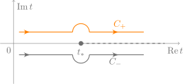
\[\begin{equation} \int_{0}^{\infty+i0}\frac{e^{-t}dt}{1-xt} -\int_{0}^{\infty-i0}\frac{e^{-t}dt}{1-xt} = \frac{2\pi i}{x}\,e^{-1/x}. \label{eq:euler-jump} \end{equation}\]
The series \(\sum n!x^n\) has real coefficients and no imaginary part to any order, yet its Borel sum is ambiguous by an imaginary amount \(e^{-1/x}\). That amount vanishes faster than any power of \(x\), which is why no finite truncation of the series can detect it.
Our integral does the same thing when we turn the coupling around. Set \(g=-\lambda\) with \(\lambda>0\). Physically, the quartic term now pulls \(x\) out to infinity: \(y=0\) is a metastable minimum, and there is a barrier at \(y^2=1\) of height
\[\begin{equation} S_{\text{barrier}} = \frac{1}{2}-\frac{1}{4}=\frac14 \qquad\text{for}\qquad S(y)=\frac{y^2}{2}-\frac{y^4}{4}. \label{eq:barrier} \end{equation}\]
The series Eq. \(\eqref{eq:series}\) becomes non-alternating, since \(a_n(-\lambda)^n\) all have the same sign. In the Borel integral, rotate \(t\to-t\) so that the kernel \(e^{-t/\lambda}\) decays again:
\[\begin{equation} Z(-\lambda) = \frac{1}{\sqrt{\pi\lambda}}\int_0^\infty e^{-t/\lambda}\,t^{-1/2}\,\widetilde{\mathcal B}(-t)\,dt . \label{eq:Z-neg} \end{equation}\]
The singularity of \(\widetilde{\mathcal B}\) at \(t=-1/4\) now sits at \(t=+1/4\), on the path. It is the barrier Eq. \(\eqref{eq:barrier}\), and the two laterals of Figure 5 now run along a cut. Past it \(\sqrt{1-4t}\) is imaginary and its sign depends on which side of the cut we pass. Near the branch point,
\[\begin{equation} \widetilde{\mathcal B}(-t) \simeq \frac{1}{\sqrt{2(1-4t)}}, \qquad \operatorname{Im}\widetilde{\mathcal B}(-t\pm i0) \simeq \mp\frac{1}{\sqrt{2(4t-1)}}\quad (t>\tfrac14), \label{eq:branch} \end{equation}\]
and the integral of the imaginary part from \(t=1/4\) gives
\[\begin{equation} \operatorname{Im} Z(-\lambda\pm i0) \simeq \mp\frac{1}{\sqrt{\pi\lambda}}\int_{1/4}^\infty \frac{e^{-t/\lambda}\,dt}{\sqrt t\,\sqrt{2(4t-1)}} \simeq \mp\frac{1}{\sqrt2}\,e^{-1/(4\lambda)} . \label{eq:imZ} \end{equation}\]
The ambiguity is \(e^{-S_{\text{barrier}}/\lambda}\). It is the tunneling amplitude through the barrier: the integral over a metastable vacuum acquires an imaginary part, and \(\operatorname{Im}Z\) is the decay rate. The numerical integral of the exact discontinuity agrees with Eq. \(\eqref{eq:imZ}\) to 1.4% at \(\lambda=0.02\), and the error shrinks linearly in \(\lambda\), as it should for a leading-order estimate.
Perturbation theory around \(y=0\) knew nothing about the barrier. The Borel transform found it anyway.
Resurgence: the series knew all along
There is a second way to see that the tunneling term and the factorial growth are the same fact. Up to now \(g\) was a number, the coupling. The integral Eq. \(\eqref{eq:Z}\) already defines \(Z\) as a function of a complex variable: that is what we used when we set \(g=-\lambda\). Once \(Z\) is a function, the coefficients \(a_n\) are not a new physical integral over couplings. They are the numbers Cauchy’s formula reads off a small circle around \(g=0\) in the complex \(g\)-plane. \(Z\) is analytic in the cut plane \(\mathbb C\setminus(-\infty,0]\), so that circle can be pushed out until it wraps the cut on the negative axis (Figure 6). The large arc at infinity vanishes, and only the discontinuity we just computed survives: both lips of the cut are \(g=-\lambda\), and \(\lambda\) is a dummy name for \(|g|\) along the cut.
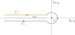
\[\begin{equation} a_n = \frac{1}{2\pi i}\oint\frac{Z(g)}{g^{n+1}}\,dg = \frac{(-1)^{n+1}}{\pi}\int_0^\infty \frac{\operatorname{Im}Z(-\lambda+i0)}{\lambda^{n+1}}\,d\lambda . \label{eq:dispersion} \end{equation}\]
This relation is exact: with the exact discontinuity in place of the approximation Eq. \(\eqref{eq:imZ}\), it returns \(a_2=105/32\) and \(a_6=23!!/(4^6\,6!)\approx 1.0723\times10^5\) to quadrature accuracy. At large \(n\) the integral is dominated by small \(\lambda\), where Eq. \(\eqref{eq:imZ}\) is accurate, with the upper sign for the upper side of the cut. Using \(\int_0^\infty e^{-1/(4\lambda)}\lambda^{-n-1}d\lambda=4^n\,\Gamma(n)\),
\[\begin{equation} a_n \simeq \frac{(-4)^n\,\Gamma(n)}{\pi\sqrt2} \qquad (n\to\infty). \label{eq:large-order} \end{equation}\]
Check it against the exact coefficients Eq. \(\eqref{eq:an}\): the ratio of the two is \(0.981\) at \(n=10\), \(0.991\) at \(n=20\), and \(0.995\) at \(n=40\). The corrections are \(1/n\) suppressed, and they come from the subleading terms in Eq. \(\eqref{eq:imZ}\).
This is what resurgence means. The coefficients of the perturbative expansion, in their large-order behavior, contain the nonperturbative tunneling sector:
- the growth rate \(4^n\) is \(1/S_{\text{barrier}}\),
- the factorial \(\Gamma(n)\) is the statement that the effect is \(e^{-S/\lambda}\) and not a power of \(\lambda\),
- the \(1/\sqrt2\) in the prefactor is \(1/\sqrt{|S''|}\) at the barrier top \(y^2=1\), the Gaussian fluctuation factor around the saddle, and the \(1/\pi\) is the dispersion relation itself.
Running the argument in reverse, the subleading corrections to Eq. \(\eqref{eq:large-order}\) encode the perturbative series around the saddle. Each sector of the theory is resurrected from the divergence of the others, which is where Écalle’s name for the subject comes from [5].
The complete answer is therefore not a power series but a trans-series,
\[\begin{equation} Z(g) = \sum_n a_n g^n \;+\; \sigma\,e^{-S/g}\,g^{\beta}\sum_n c_n g^n \;+\;\cdots , \label{eq:transseries} \end{equation}\]
where the constant \(\sigma\) jumps when \(\arg g\) crosses a Stokes line, by exactly the amount needed to cancel the jump Eq. \(\eqref{eq:imZ}\) of the lateral Borel sums. The two ambiguities, one from resumming perturbation theory and one from choosing which saddles to include, cancel. For the stable integral Eq. \(\eqref{eq:Z}\) with \(g>0\), the saddles at \(y=\pm i\) do not contribute (\(\sigma=0\)), and the plain Borel sum is the whole answer, as we found.
Remarks
In the double-well potential the situation is the one we just saw for \(g<0\), but now in the physical region. The ground-state energy has a non-Borel-summable perturbation series. The instanton–anti-instanton contribution has an imaginary part that is also ambiguous. The two imaginary parts cancel exactly, leaving a real energy [6], [7]. The same mechanism is now used to give meaning to perturbation series in quantum field theory and string theory [8].
The move that made all of it possible was the one that looked stupid: throwing away \(n!\) and then putting it back as \(\int t^n e^{-t}dt\). It turned out to be the change of measure from \(dy\) to \(dS\), from the field to the action. The Borel plane is the plane of actions, and its singularities are the saddles that perturbation theory forgot.
References
[1]
F. J. Dyson, “Divergence of perturbation theory in quantum electrodynamics,” Physical Review, vol. 85, pp. 631–632, 1952, doi: 10.1103/PhysRev.85.631.
[2]
C. M. Bender and T. T. Wu, “Anharmonic oscillator,” Physical Review, vol. 184, pp. 1231–1260, 1969, doi: 10.1103/PhysRev.184.1231.
[3]
M. Mariño, “An introduction to resurgence in quantum theory.” 2023.
[4]
É. Borel, “Mémoire sur les séries divergentes,” Annales scientifiques de l’École Normale Supérieure, vol. 16, pp. 9–131, 1899, doi: 10.24033/asens.467.
[5]
J. Écalle, Les fonctions résurgentes. Orsay: Publications Mathématiques d’Orsay, 1981.
[6]
E. B. Bogomolny, “Calculation of instanton–anti-instanton contributions in quantum mechanics,” Physics Letters B, vol. 91, pp. 431–435, 1980, doi: 10.1016/0370-2693(80)90538-6.
[7]
J. Zinn-Justin and U. D. Jentschura, “Multi-instantons and exact results I: Conjectures, WKB expansions, and instanton interactions,” Annals of Physics, vol. 313, pp. 197–267, 2004, doi: 10.1016/j.aop.2004.04.004.
[8]
D. Dorigoni, “An introduction to resurgence, trans-series and alien calculus,” Annals of Physics, vol. 409, p. 167914, 2019, doi: 10.1016/j.aop.2019.167914.
Footnotes
The last integral is a Laplace transform in disguise: the substitution \(u=gt\) gives \(Z(g)=g^{-1}(\mathcal L\mathcal B)(1/g)\), so \(g\) is the inverse of the Laplace variable.↩︎