Laser speckle, the Rice distribution, and photon statistics
laser speckle, Rice distribution, photon counting, interarrival times, statistical speckle discrimination
Introduction
When laser light reflects from a rough surface or propagates through a turbid medium, the wave at a given point is a sum of many contributions with random optical paths. Most of the field can be viewed as a strong coherent background phasor (specular or ballistic component) plus weak scattered phasors whose phases wander. Interference among those random terms produces the familiar granular speckle intensity pattern.
The same mathematical picture applies in other coherent-imaging settings. In coronagraphy, for example, a small amount of starlight scatters into the focal plane and creates speckles that mimic faint companions. Stochastic Speckle Discrimination (SSD) separates a true incoherent source from speckle by comparing their statistics: speckle-dominated modes behave like a biased coherent random field (Rice statistics on amplitude), whereas photons from a faint companion are often well modeled as Poisson in each integration.
This post develops the classical field side first (transformations of random variables, then the Rice law for amplitude), and then connects the field to intensity and photon arrivals, including interarrival times, so the Poisson-versus-speckle contrast is visible at the level of counting statistics as well as Fourier or spatial modes.
Notes on Functions of Random Variables
We will need certain transformations of random variables. This will require some basic knowledge of probability theory and functions of random variables. In the standard notation, a random variable is denoted by a capital letter, and its value is denoted by a lowercase letter. For example, \(U\) is a random variable, and \(u\) is its value. Assume we know that \(U\) has a probability density function \(f_U(u)\). This random variable is subject to a transformation \(V = g(U)\), where \(g\) is a known function. We want to find the probability density function of the new random variable \(V\), denoted as \(f_V(v)\).
The cumulative distribution function of the transformed random variable \(V\) is given by:
\[\begin{equation} F_V(v) = P(V \leq v) \label{eq:cumulative_distribution_function}. \end{equation}\] An illustration of this transformation is shown in Figure 1. The domain of \(v\leq V\) is mapped to the domain of \(u\) as shown in green line segments on the x-axis. Let us define this domain as \(L_v\).
We can express \(\ref{eq:cumulative_distribution_function}\) in terms of \(u\) \[\begin{equation} F_V(v) = P(V \leq v) = P( U \in L_v) \label{eq:cumulative_distribution_function_in_terms_of_u}. \end{equation}\]
The probability density function of the transformed random variable \(V\) is given by:
\[\begin{equation} f_V(v) = \frac{d}{dv} F_V(v) = \frac{d}{dv} P( U \in L_v) \label{eq:probability_density_function_of_v}. \end{equation}\]
In the general case, we need to find the domains (\(L_v\)) and compute the derivative in \(\ref{eq:probability_density_function_of_v}\). Let’s start with an example:
\[\begin{equation} g(u) =a u^2 \label{eq:gofu}. \end{equation}\]
\[\begin{equation} F_V(v) = P(V \leq v) = P( U \in L_v)=P(-\sqrt{\frac{v}{a}} \leq u \leq \sqrt{\frac{v}{a}}) =\int_{-\sqrt{\frac{v}{a}}}^{\sqrt{\frac{v}{a}}} f_U(u) du \label{eq:cumulative_distribution_function_in_terms_of_usq}. \end{equation}\]
\[\begin{eqnarray} f_V(v) &=& \frac{d}{dv} F_V(v) = \left\{f_U\left(\sqrt{\frac{v}{a}}\right) +f_U\left(-\sqrt{\frac{v}{a}}\right) \right\} \left[\frac{d}{dv}\sqrt{\frac{v}{a}}\right]\nonumber\\ &=& \frac{f_U\left(\sqrt{\frac{v}{a}}\right) +f_U\left(-\sqrt{\frac{v}{a}}\right)} {2\sqrt{a v}} \label{eq:probability_density_function_of_v_sq}. \end{eqnarray}\]
For example, if \(f_U\) is a uniform distribution, \(f_U(u) = \frac{1}{c-b}\) for \(u \in [b,c]\), then under the transformation \(a\,v^2\), the domain gets mapped to \([a\,b^2,a\,c^2]\). Inserting this into \(\ref{eq:probability_density_function_of_v_sq}\) we get:
\[\begin{equation} f_V(v) = \begin{cases} \frac{1}{2\sqrt{a v} (c-b)}, & b^2<v<c^2 \\ 0, & \text{otherwise} \end{cases} \label{eq:probability_density_function_of_v_sq_uniform}, \end{equation}\] which is shown in Figure 3.
One may be concerned about the singularity at \(v=0\). It is still integrable, and the probability function is well defined. We can show that the normalization still holds after the transformation.
\[\begin{equation} \int_{-\infty}^{\infty} dv f_V(v) = \int_{a\,b^2}^{a\,c^2} \frac{dv}{2\sqrt{a v} (c-b)} = \frac{1}{\sqrt{a} (c-b)}\left.\sqrt{v} \right|_{a\,b^2}^{a\,c^2} = 1 \label{eq:probability_density_function_of_v_sq_uniform_normalization}, \end{equation}\]
The same squaring map appears when we pass from a complex amplitude to intensity \(I \propto |V|^2\) in Section 3: if the field component along some quadrature behaves like a random variable, its square drives the intensity distribution.
Statistics of the wave amplitude
We describe the scalar field (one polarization, one narrowband mode) as a random vector in the complex plane. A deterministic phasor models the coherent laser carrier that survives specular reflection or ballistic transmission; random fluctuations represent diffuse scattering from surface roughness, bulk heterogeneity, or multiple paths with different phases. Figure 4 illustrates the geometry: a fixed phasor \(V_0\) plus steps that accumulate speckle noise.
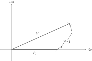
We can express the resultant phasor as a sum of a deterministic phasor and a collection of random phasors: \[\begin{equation} V=V_0+\frac{1}{\sqrt{N}}\sum_{i=1}^{N} \alpha_i e^{i\phi_i}, \label{eq:resultant_v} \end{equation}\] where \(V_0\) is the coherent bias phasor, \(\alpha_i\) and \(\phi_i\) are the amplitudes and phases of the scattered contributions, respectively. Individual scatterers are taken to be independent.
We will assume that \(\alpha_i\) are i.i.d. random variables with mean \(\bar{\alpha}\) and variance \(\sigma_{\alpha}^2\). We can define the real and imaginary parts of the resultant phasor as: \[\begin{equation} \Re \{V\}=V_{0r}+\frac{1}{\sqrt{N}}\sum_{i=1}^{N} \alpha_i \cos(\phi_i), \label{eq:resultant_v_r} \end{equation}\] \[\begin{equation} \Im \{V\}=V_{0i}+\frac{1}{\sqrt{N}}\sum_{i=1}^{N} \alpha_i \sin(\phi_i) \label{eq:resultant_v_i}, \end{equation}\]
The expected value of the real and imaginary parts of the resultant phasor are simply set by the deterministic phasor: \[\begin{equation} \langle\Re \{V\} \rangle = \Re \{V_0\} \label{eq:resultant_v_r_mean}, \end{equation}\] \[\begin{equation} \langle \Im \{V\} \rangle = \Im \{V_0\} \label{eq:resultant_v_i_mean}. \end{equation}\]
We can also compute the variance: \[\begin{equation} \langle\left(\Re \{V\}-\langle\Re \{V\} \rangle\right)^2 \rangle =\langle\left(\Re \{V\}-\Re \{V_0\}\right)^2 \rangle = \frac{1}{N}\sum_{i=1}^{N} \int d \alpha_i \int (\alpha_i-\bar\alpha)^2 d \phi_i \cos^2(\phi_i) =\frac{\sigma_{\alpha}^2}{2}\equiv \sigma^2 \label{eq:resultant_v_r_variance}. \end{equation}\]
By symmetry, the imaginary part has the same variance after subtracting its mean: \(\langle(\Im\{V\}-\langle\Im\{V\}\rangle)^2\rangle=\sigma^2\). We may rotate coordinates so that \(V_0\) lies on the real axis. Then the means become \[\begin{equation} \langle\Re \{V\} \rangle = \Re \{V_0\}\equiv s \label{eq:resultant_v_r_meanr}, \end{equation}\] \[\begin{equation} \langle \Im \{V\} \rangle \equiv 0 \label{eq:resultant_v_i_meanr}. \end{equation}\]
As the vector is composed of many random phasors, the resultant vector will be a Gaussian distribution due to the central limit theorem. We have computed its mean and variance. We can put them into the normal distribution:
\[\begin{equation} f_{R,I}(r,i) =\frac{1}{2\pi \sigma^2} \exp\left(-\frac{(r-s)^2+i^2}{2\sigma^2}\right) \label{eq:resultant_gaussian}, \end{equation}\] where we denote the real and imaginary parts of the resultant vector as \(r\) and \(i\), respectively.
This is the representation of the resultant vector in the Cartesian coordinate system \((r,i)\). We can transform it into the polar coordinate system \((A,\Theta)\):
\[\begin{equation} \begin{aligned} a &= \sqrt{r^2+i^2} \\ \theta &= \tan^{-1}\left(\frac{i}{r}\right) \end{aligned} \quad\iff\quad \begin{aligned} r &= a \cos \theta \\ i &= a \sin \theta \end{aligned} \label{eq:resultant_polar_inverse} \end{equation}\] Transforming the probability density function of the resultant vector from Cartesian to polar coordinates, we get: \[\begin{equation} f_{A,\Theta}(a,\theta) =\begin{cases} \frac{a}{2\pi \sigma^2} \exp\left(-\frac{(a \cos \theta-s)^2+(a \sin \theta)^2}{2\sigma^2}\right), & a\geq 0 \text{ and } -\pi<\theta<\pi \\ 0, & \text{otherwise} \end{cases} \label{eq:resultant_polar_pdf} \end{equation}\] where \(a\) factor comes from the Jacobian of the transformation.
In order to find the probability density function of the amplitude, we need to integrate over the angle \(\theta\): \[\begin{eqnarray} f_A(a) &=& \int_{-\pi}^{\pi} f_{A,\Theta}(a,\theta)\, d\theta = \frac{a}{2\pi \sigma^2} \exp\left(-\frac{a^2 +s^2}{2\sigma^2}\right) \int_{-\pi}^{\pi} \exp\left(-\frac{a s \cos \theta}{\sigma^2}\right) d\theta\\ &=& \frac{a}{\sigma^2} \exp\left(-\frac{a^2 +s^2}{2\sigma^2}\right) I_0\left(\frac{a s}{\sigma^2}\right) \label{eq:resultant_polar_pdf_a}, \end{eqnarray}\] using \(\int_{-\pi}^{\pi} e^{z\cos\theta}\,d\theta = 2\pi I_0(z)\) with \(z=as/\sigma^2\). Here \(I_0\) is the modified Bessel function of the first kind.
\[\begin{eqnarray} f_A(a) &=& \begin{cases} \dfrac{a}{\sigma^2} \exp\left(-\dfrac{a^2 +s^2}{2\sigma^2}\right) I_0\left(\dfrac{a s}{\sigma^2}\right), & a\geq 0 \\ 0, & \text{otherwise.} \end{cases} \label{eq:resultant_polar_pdf_a2} \end{eqnarray}\] This is the standard Rice form (often written with \(a/\sigma^2\) rather than \(a/(2\pi\sigma^2)\) after normalizing the angular marginal); \(I_0\) is the modified Bessel function of the first kind. Figure 5 plots \(f_A(a)\) for several ratios \(s/\sigma\).
Intensity and photon arrivals
Up to a detector proportionality constant, the instantaneous intensity is \(I = |V|^2\). With the polar amplitude \(A=a\) from Section 2, we have \(I=a^2\) and may write the intensity cdf as \(F_I(x)=P(I\le x)=P(A\le \sqrt{x})=F_A(\sqrt{x})\) for \(x\ge 0\). Differentiating, \[\begin{equation} f_I(x) = \frac{d}{dx}F_A(\sqrt{x}) = \frac{f_A(\sqrt{x})}{2\sqrt{x}}, \qquad x>0, \label{eq:intensity_from_amplitude} \end{equation}\] which is the same Jacobian factor as in the squaring map \(u\mapsto a u^2\) treated earlier.
When \(s=0\) (pure circular Gaussian field, fully developed speckle with no coherent bias), \(f_A(a)=\frac{a}{\sigma^2}\exp(-a^2/(2\sigma^2))\) and \(\ref{eq:intensity_from_amplitude}\) yields the negative exponential intensity law \(f_I(x)=\frac{1}{2\sigma^2}\exp(-x/(2\sigma^2))\) on \(x>0\). When \(s>0\), the intensity pdf is peaked away from zero: the coherent offset breaks the “dark core” of Rayleigh speckle.
Photon counts in a short window
Let \(\tau\) be an integration time short enough that \(I\) is approximately constant, but long enough to register many photons in bright conditions. Semiclassical photon counting says that, conditional on \(I\), the number detected is Poisson: \[\begin{equation} P(N=n \mid I) = \frac{(\lambda(I)\,\tau)^n}{n!}\, e^{-\lambda(I)\,\tau}, \qquad n=0,1,2,\ldots \label{eq:poisson_conditional} \end{equation}\] with a rate proportional to intensity, \(\lambda(I)=\eta I\) for some efficiency \(\eta>0\).
If \(I\) is fixed (steady incoherent source, or a laser speckle grain that does not move on the time scale of interest), then \(\ref{eq:poisson_conditional}\) is ordinary Poisson with a constant mean \(\bar N = \eta I \tau\). The Fano factor \(\mathcal{F}=\mathrm{Var}(N)/\mathbb{E}[N]\) equals one.
If instead \(I\) is random—for example because the pixel samples a speckle field that changes with wavelength, scatterer motion, or atmospheric evolution—then we must average \(\ref{eq:poisson_conditional}\) over the statistics of \(I\). The mean is \(\mathbb{E}[N]=\eta\tau\,\mathbb{E}[I]\), but \[\begin{equation} \mathrm{Var}(N) = \mathbb{E}[\mathrm{Var}(N\mid I)] + \mathrm{Var}(\mathbb{E}[N\mid I]) = \mathbb{E}[\lambda(I)\tau] + (\eta\tau)^2\,\mathrm{Var}(I), \label{eq:fano_doubly_stochastic} \end{equation}\] so whenever \(\mathrm{Var}(I)>0\), \[\begin{equation} \mathcal{F} = 1 + \frac{\eta\tau\,\mathrm{Var}(I)}{\mathbb{E}[I]} > 1. \label{eq:fano_gt_one} \end{equation}\] Such doubly stochastic (or compound Poisson) counting is super-Poissonian: relative fluctuations exceed those of a Poisson process with the same mean.
Interarrival times
For a homogeneous Poisson process with constant rate \(\lambda\), the waiting time \(T\) until the next count satisfies \[\begin{equation} P(T>t) = e^{-\lambda t}, \qquad f_T(t)=\lambda e^{-\lambda t}, \quad t\ge 0, \label{eq:exponential_interarrival} \end{equation}\] the exponential interarrival density.
When the effective rate \(\lambda(I(t))\) fluctuates in time because speckle intensity drifts or because different samples draw different speckle realizations, the unconditional gap distribution is no longer a single exponential (\(\ref{eq:exponential_interarrival}\)): the mixture of exponentials with different rates produces heavier or structured tails. By contrast, a weak thermal or incoherent point source that delivers a steady Poisson stream at the detector exhibits exponential gaps at fixed intensity. Comparing Fano factors, variance-to-mean of binned counts, or interarrival summaries is therefore one route to statistical speckle discrimination—the same logical contrast as in SSD, where a companion’s photons follow Poisson-like counting in a mode while speckle-contaminated modes inherit the higher variability of a random classical intensity.
Discussion
The Rice law describes field-level speckle when a coherent bias is present; intensity is a monotone map of amplitude, and photon statistics inherit randomness from intensity whenever that intensity varies across the ensemble or in time. An idealized CW laser illuminating a static rough surface can still yield temporal Poisson arrivals at each fixed pixel because the classical rate is constant; discrimination then relies on spatial or spectral diversity, dynamic speckle, or the presence of a separate incoherent component—not every laboratory speckle pattern violates (\(\ref{eq:exponential_interarrival}\)).
Stochastic Speckle Discrimination in coronagraphy uses the same idea in Fourier or mode space: statistics of the speckle field differ from those of a faint physical source. The mathematics in this note is portable between laser speckle in the lab and starlight speckle on a telescope.