Computing joint confidence intervals
Normal distribution, confidence intervals, central limit theorem, statistical inference
Introduction
The goal is to combine information from separate experimental runs to quote a single number to assess the difference of two groups in the data. This would be a case where one cannot combine the data sets due to confounding factors. We will discuss two ways of combining statistics:
- Computing joint \(p\)-values,
- Computing joint confidence intervals.
Sampling statistics
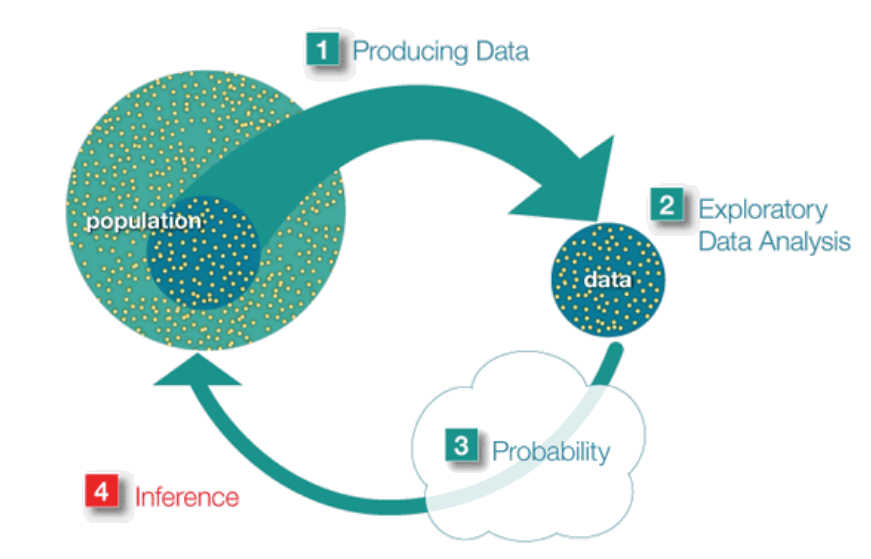
The end goal of statistics is to estimate the true values of the population parameters, such as the mean value \(\mu\) and the variance \(\sigma^2\). We try to get a sense of what \(\mu\) could be by pulling \(N\) samples from the population and studying it. Each sample is a random variable, \(S_i\), and we can compute their average
\[\begin{eqnarray} \bar S=\frac{1}{N}\sum_{i=1}^{N}S_i. \label{eq:avg} \end{eqnarray}\] \(S\) itself is a random variable: it will be different if you pick up another set of \(N\) samples. We can also compute its expected value \[\begin{eqnarray} E[\bar S]=\frac{1}{N}\sum_{i=1}^{N} E[S_i]=\mu , \label{eq:eavg} \end{eqnarray}\] and its variance \[\begin{eqnarray} \text{Var}[\bar S]=\frac{1}{N^2}\sum_{i=1}^{N} \text{Var}[S_i]=\frac{\sigma^2}{N}. \label{eq:var} \end{eqnarray}\] Furthermore, by central limit theorem, we know that for large \(N\) \(\bar S\) will be normally distributed, denoted as \[\begin{eqnarray} \bar S \sim \mathcal{N}\left(\mu,\frac{\sigma^2}{N}\right). \label{eq:snormal} \end{eqnarray}\]
\(p\)-Values
The P value is the probability of obtaining a result equal to or larger than what was actually observed assuming the null hypothesis is true. It does not give the probability of the null hypothesis is true or not. Figure 1 illustrates the \(p-\)value.

Such a number can be computed for any distribution and should be compared against \(\alpha\), which determines how extreme the data must be for the null hypothesis to be rejected. For example, for \(\alpha=5\%\), \(p<0.05\) will result in the rejection of the null hypothesis.
Pooling \(p-\)values
A way of pooling \(p-\)values is proposed in [1] as a harmonic sum \[\begin{eqnarray} \frac{1}{\bar p}=\frac{\sum_{i=1}^n{\frac{Ni}{p_i}}}{\sum_{i=1}^n N_i} \label{eq:pbarl} \end{eqnarray}\] where \(N_i\)’s are the samples sizes, and \(p_i\)’s are the individual \(p-\)values computed for each experiment, and \(n\) is the number of experiments to be pooled. For equal sample sizes, this simplifies to \[\begin{eqnarray} \frac{1}{\bar p}=\frac{\sum_{i=1}^n{\frac{1}{p_i}}}{n} \label{eq:pbarle} \end{eqnarray}\] This will result in a single number that will represent the results combining from all experimental runs.
Confidence intervals
When the true values of the population parameters, \(\mu\) and \(\sigma^2\) are unknown, we can replace them with the sample statistics \(\hat{\mu}\) and \(\hat\sigma^2\) \[\begin{eqnarray} \bar S \sim \mathcal{N}\left(\hat\mu,\frac{\hat\sigma^2}{N}\right). \label{eq:snormalsample} \end{eqnarray}\] We are trying to estimate \(\mu\) and \(\sigma^2\) based on the data we sample. This is illustrated in Figure 2.
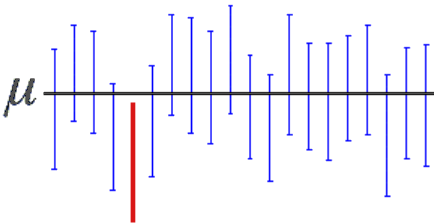
Equation \(\ref{eq:snormalsample}\) tells us that the sample mean value, \(\hat \mu\), will vary from as we get another set of \(N\) samples. And we do not necessarily know its relative position with respect to the population mean \(\mu\). We want to create an interval around the \(\hat \mu\) such that we can estimate whether \(\mu\) will happen to be in that interval. It is important to notice that this is more about creating a procedure to create an interval which, if repeated, will contain the population mean value \(\mu\). Assume you have a method of creating confidence intervals(CI), say with \(95\%\) confidence, which we will discuss later, below is what it means:
- You pull \(N\) samples and compute the interval with the data.
- \(\mu\) is not guaranteed to be in the interval.
- You cannot say it will be in the interval with \(95\%\) probability. It is either in or out. This is not probabilistic.
- You go back and pull \(N\) new samples.
- Note that you will have a new \(\hat\mu\) and a new confidence interval. \(\mu\) may or may not be in it.
- If you repeat the process many times, if your method of computing intervals is correct, \(95\%\) of the intervals you computed will include the true value \(\mu\).
- The process is illustrated in Figure 3.
To compute the confidence intervals, it is convenient to define the following random variable: \[\begin{eqnarray} Z=\frac{\bar S-\hat\mu}{\frac{\hat\sigma}{\sqrt{N}}} \label{eq:z} \end{eqnarray}\] If the sample size is large (\(N>\sim30\)), this particular random variable will have standard normal distribution1. A confidence level of \(c\) corresponds to a \(z^*\) value such that the area under the standard normal distribution between \(-z^*\) and \(z^*\) is \(c\). Equivalently, the area outside on each side will be \(\frac{1-c}{2}=\frac{\alpha}{2}\), where \(\alpha\equiv1-c\). Take an example of \(95\%\) confidence level, which yields \(\alpha=0.05\). The value of \(z^*\) in this case will be \(1.96\) so that \(2.5\%\) of the total area lies under each tail, i.e., \(|z|>1.96\). Rearranging Eq. \(\ref{eq:z}\) shows that \(95\%\) CI is from \(\hat\mu-1.96\frac{\hat\sigma}{\sqrt{N}}\) to \(\hat\mu+1.96\frac{\hat\sigma}{\sqrt{N}}\). Figure 3 shows this for generic \(c\).

A confidence interval with confidence level \(c\) is constructed by finding the critical values \(\pm z_{\alpha/2}\) such that the area under the standard normal distribution between these values equals \(c\). The remaining area \(\alpha = 1-c\) is split equally between the two tails, with each tail containing area \(\alpha/2\).
Pooling multiple confidence levels
Assume you have two sets of data, and you can compute \(\hat \mu\), \(\hat \sigma\) and the corresponding CIs for each set of data. How would you combine these two sets to produce joint CIs? We can do this by pooling the estimates as follows:
\[\begin{eqnarray} \bar S=\frac{N_1 \bar S_1+N_2 \bar S_2}{N_1+N_2} \label{eq:pool} \end{eqnarray}\] where subscripts label the data sets. \(\bar S\) is yet another normal random variable, and we can compute its expected value as \[\begin{eqnarray} E[\bar S]=\frac{N_1 \hat\mu_1+N_2 \hat\mu_2}{N_1+N_2} , \label{eq:eavgj} \end{eqnarray}\] and its variance: \[\begin{eqnarray} \text{Var}[\bar S]=\frac{N_1^2 \text{Var}[\bar S_1]+N_2^2 \text{Var}[\bar S_2]}{(N_1+N_2)^2}=\frac{N_1^2 \frac{\hat\sigma_1^2}{N_1}+N_2^2 \frac{\hat\sigma_2^2}{N_2}}{(N_1+N_2)^2}=\frac{N_1 \hat\sigma_1^2+N_2\hat\sigma_2^2}{(N_1+N_2)^2}. \label{eq:varj} \end{eqnarray}\] Therefore, the pooled estimator becomes \[\begin{eqnarray} \bar S \sim \mathcal{N}\left(\frac{N_1 \hat\mu_1+N_2 \hat\mu_2}{N_1+N_2},\frac{N_1 \hat\sigma_1^2+N_2\hat\sigma_2^2}{(N_1+N_2)^2}\right), \label{eq:snormalj} \end{eqnarray}\] which completely defines the joint distribution. One can easily compute the corresponding CI as \[\begin{eqnarray} \left[\frac{N_1 \hat\mu_1+N_2 \hat\mu_2}{N_1+N_2}-z_{\frac{\alpha}{2}}\frac{\sqrt{N_1 \hat\sigma_1^2+N_2\hat\sigma_2^2}}{N_1+N_2},\frac{N_1 \hat\mu_1+N_2 \hat\mu_2}{N_1+N_2}+z_{\frac{\alpha}{2}}\frac{\sqrt{N_1 \hat\sigma_1^2+N_2\hat\sigma_2^2}}{N_1+N_2}\right]. \label{eq:cij} \end{eqnarray}\] For equal sample sizes, \(N_1=N_2=N\), we get \[\begin{eqnarray} \left[\frac{\hat\mu_1+\hat\mu_2}{2}-z_{\frac{\alpha}{2}}\frac{\sqrt{ \hat\sigma_1^2+\hat\sigma_2^2}}{2},\frac{\hat\mu_1+\hat\mu_2}{2}+z_{\frac{\alpha}{2}}\frac{\sqrt{ \hat\sigma_1^2+\hat\sigma_2^2}}{2}\right], \label{eq:cijeq} \end{eqnarray}\] which is the final result expressing the CI in terms of the statistical parameters of both experiments.
Visualization
Below you can change the statistics of two samples and observe how the joint distribution behaves. Note that these curves represent the inferred distribution of the mean of the samples as described in Eqs. \(\ref{eq:snormalsample}\) and \(\ref{eq:snormalj}\), not to be confused with the distribution of data points in each sample.
References
Footnotes
for \(N<\sim 30\), it will be \(t\)-distribution. Here we will assume sample size is large enough↩︎